GensimによるWord2Vecの学習と使用#

前章でCBOWモデルを実装することでword2vecの仕組みを学びました。実際に、その以外、word2vecの関して様々な取り組みがあります。

Skip-gramモデルでは、ターゲットからコンテキストを推測するタスクを構築しています
Negative Samplingという新しい損失関数を導入することで学習の高速化を図る

応用の視点から、これらの手法をすべでゼロから実装することが難しいので、gensimというライブラリを使って、Word2Vecモデルを学習、管理、使用することは、多くの自然言語処理タスクにおいて効果的な選択肢となります。

#!pip install --upgrade gensim

Gensimの使い方#

Gensimによる学習#

from gensim.models import Word2Vec

sample_sents = [['you', 'say', 'goodbye', 'and', 'I', "say", "hello" '.']]
model = Word2Vec(sentences=sample_sents, vector_size=5, window=1, min_count=1)

model.wv['you']

array([-0.06810732, -0.01892805,  0.11537147, -0.15043278, -0.0787221 ],
      dtype=float32)

オプション	説明
sentences	元となるコーパス．単語リストのリスト．
corpus_file	コーパスをファイル読み込みする場合に指定．1行1文の形式で，単語は空白区切りで認識される．
vector_size	分散表現の次元．リファレンスではvector_sizeと書いてあるように見えるが，sizeでないと動かない．
window	学習時に利用されるコンテキストの長さ．
min_count	分散表現を獲得する単語の最小頻度
workers	学習時の使用スレッド数．
sg	学習アルゴリズムの選択．\(1\)ならskip-gram，\(0\)ならCBOW．

with open('./Data/lee_background.cor', 'r') as file:
    corpus = file.readlines()

processed_corpus = [line.lower().split() for line in corpus]

model = Word2Vec(sentences=processed_corpus, vector_size=100, window=5, min_count=5)

課題

ドキュメントを参照しながら、以下の指示に従ってモデルを実装してください。

コーパスファイルパスを指定する形でコーパスを導入しなさい
学習方法はskip-gramを使う
negative samplingを使う

Gensimによる日本語モデル学習#

import MeCab
def tokenize(text):
    """ テキストを形態素解析して、トークンのリストを返す """
    mecab = MeCab.Tagger("-Owakati")
    return mecab.parse(text).strip().split()

documents = ["これはサンプルの文書です。", "Word2Vecの学習を行います。"]

# 形態素解析を行い、単語リストに変換
tokenized_documents = [tokenize(doc) for doc in documents]

# Word2Vecモデルの訓練

model_jp = Word2Vec(sentences=tokenized_documents, vector_size=100, window=5, min_count=1, workers=4)

モデルの使い方#

モデルには,wvというオブジェクトに単語と単語分散表現の情報が格納されています。さらに、学習済みの単語ベクトルにアクセスし、それらを操作するための主要なインターフェースを提供します。

単語ベクトルの取得: model.wv['word'] で特定の単語のベクトルを取得できます。

model.wv['you']

array([ 0.01955878,  0.23760737,  0.08624359,  0.23176762,  0.07768093,
       -0.7730639 ,  0.29753113,  0.9506419 , -0.36420536, -0.45274746,
       -0.28820178, -0.6818679 , -0.27447   ,  0.07585317,  0.16149026,
       -0.23213369,  0.1356584 , -0.18800561,  0.14164801, -0.90509045,
        0.21500997,  0.19327609,  0.43587556, -0.14708444, -0.15819708,
       -0.14492755, -0.52023107, -0.12544046, -0.39281872,  0.07534824,
        0.597077  , -0.11641099,  0.37067735, -0.7197579 , -0.06213377,
        0.34813905,  0.1539449 , -0.35367858, -0.4453832 , -0.6412594 ,
        0.14452343, -0.3251846 , -0.40699026,  0.27088606,  0.2807835 ,
       -0.22798546, -0.4351668 , -0.11758936,  0.24796194,  0.3342767 ,
        0.23265927, -0.30068317, -0.23268035, -0.19075954, -0.2161348 ,
       -0.02259099,  0.18425396, -0.17584062, -0.43471783,  0.09690897,
       -0.08698869,  0.14127013,  0.04958015,  0.02455294, -0.59545493,
        0.56266534,  0.04993773,  0.17407547, -0.52165055,  0.3226274 ,
       -0.3517651 ,  0.26038453,  0.5212256 , -0.12726067,  0.5554784 ,
        0.09757318, -0.07757214, -0.01927667, -0.34825307,  0.03948191,
       -0.34005928, -0.04186369, -0.23001537,  0.6189364 , -0.21654902,
       -0.2240897 , -0.02051629,  0.02020353,  0.57382953, -0.01938878,
        0.6551917 ,  0.37754795,  0.07158637,  0.06285442,  0.7467078 ,
        0.300077  ,  0.09780832, -0.09670246,  0.12873173, -0.260617  ],
      dtype=float32)

類似度の計算: model.wv.similarity('word1', 'word2') で2つの単語間の類似度を計算できます。

model.wv.similarity("you", "your")

0.99931145

最も類似した単語の取得: model.wv.most_similar('word') で特定の単語に最も類似した単語を取得できます

model.wv.most_similar("you")

[('this', 0.9997767210006714),
 ('also', 0.9997580647468567),
 ('last', 0.9997541308403015),
 ('are', 0.9997477531433105),
 ('with', 0.9997434616088867),
 ('us', 0.9997416138648987),
 ('police', 0.9997385740280151),
 ('all', 0.999736487865448),
 ('were', 0.9997210502624512),
 ('some', 0.9997204542160034)]

Note

Gensimで学習済みモデルを使用する方法は、モデルの種類と読み込み方法によって異なります。通常は、通常はwvを介してベクトルにアクセスしますが、KeyedVectorsを使用する場合、KeyedVectors自体が単語ベクトルへの直接アクセスを提供するので、wvは不要です。

モデルの管理#

# モデルの保存と読み込み
#model.save("word2vec.model")
#model = Word2Vec.load("word2vec.model")

学習済みモデルの読み込み#

Gensimはいくつかの学習済みモデルを提供して、簡単に読み込むことができます。

import gensim.downloader

print(list(gensim.downloader.info()['models'].keys()))

['fasttext-wiki-news-subwords-300', 'conceptnet-numberbatch-17-06-300', 'word2vec-ruscorpora-300', 'word2vec-google-news-300', 'glove-wiki-gigaword-50', 'glove-wiki-gigaword-100', 'glove-wiki-gigaword-200', 'glove-wiki-gigaword-300', 'glove-twitter-25', 'glove-twitter-50', 'glove-twitter-100', 'glove-twitter-200', '__testing_word2vec-matrix-synopsis']

model = gensim.downloader.load('word2vec-google-news-300')

---------------------------------------------------------------------------
KeyboardInterrupt                         Traceback (most recent call last)
Cell In[15], line 1
----> 1 model = gensim.downloader.load('word2vec-google-news-300')

File /opt/anaconda3/envs/jupyterbook/lib/python3.10/site-packages/gensim/downloader.py:503, in load(name, return_path)
    501 sys.path.insert(0, BASE_DIR)
    502 module = __import__(name)
--> 503 return module.load_data()

File ~/gensim-data/word2vec-google-news-300/__init__.py:8, in load_data()
      6 def load_data():
      7     path = os.path.join(base_dir, 'word2vec-google-news-300', "word2vec-google-news-300.gz")
----> 8     model = KeyedVectors.load_word2vec_format(path, binary=True)
      9     return model

File /opt/anaconda3/envs/jupyterbook/lib/python3.10/site-packages/gensim/models/keyedvectors.py:1719, in KeyedVectors.load_word2vec_format(cls, fname, fvocab, binary, encoding, unicode_errors, limit, datatype, no_header)
   1672 @classmethod
   1673 def load_word2vec_format(
   1674         cls, fname, fvocab=None, binary=False, encoding='utf8', unicode_errors='strict',
   1675         limit=None, datatype=REAL, no_header=False,
   1676     ):
   1677     """Load KeyedVectors from a file produced by the original C word2vec-tool format.
   1678 
   1679     Warnings
   (...)
   1717 
   1718     """
-> 1719     return _load_word2vec_format(
   1720         cls, fname, fvocab=fvocab, binary=binary, encoding=encoding, unicode_errors=unicode_errors,
   1721         limit=limit, datatype=datatype, no_header=no_header,
   1722     )

File /opt/anaconda3/envs/jupyterbook/lib/python3.10/site-packages/gensim/models/keyedvectors.py:2065, in _load_word2vec_format(cls, fname, fvocab, binary, encoding, unicode_errors, limit, datatype, no_header, binary_chunk_size)
   2062 kv = cls(vector_size, vocab_size, dtype=datatype)
   2064 if binary:
-> 2065     _word2vec_read_binary(
   2066         fin, kv, counts, vocab_size, vector_size, datatype, unicode_errors, binary_chunk_size, encoding
   2067     )
   2068 else:
   2069     _word2vec_read_text(fin, kv, counts, vocab_size, vector_size, datatype, unicode_errors, encoding)

File /opt/anaconda3/envs/jupyterbook/lib/python3.10/site-packages/gensim/models/keyedvectors.py:1958, in _word2vec_read_binary(fin, kv, counts, vocab_size, vector_size, datatype, unicode_errors, binary_chunk_size, encoding)
   1955 tot_processed_words = 0
   1957 while tot_processed_words < vocab_size:
-> 1958     new_chunk = fin.read(binary_chunk_size)
   1959     chunk += new_chunk
   1960     processed_words, chunk = _add_bytes_to_kv(
   1961         kv, counts, chunk, vocab_size, vector_size, datatype, unicode_errors, encoding)

File /opt/anaconda3/envs/jupyterbook/lib/python3.10/gzip.py:301, in GzipFile.read(self, size)
    299     import errno
    300     raise OSError(errno.EBADF, "read() on write-only GzipFile object")
--> 301 return self._buffer.read(size)

File /opt/anaconda3/envs/jupyterbook/lib/python3.10/_compression.py:68, in DecompressReader.readinto(self, b)
     66 def readinto(self, b):
     67     with memoryview(b) as view, view.cast("B") as byte_view:
---> 68         data = self.read(len(byte_view))
     69         byte_view[:len(data)] = data
     70     return len(data)

File /opt/anaconda3/envs/jupyterbook/lib/python3.10/gzip.py:494, in _GzipReader.read(self, size)
    491     self._new_member = False
    493 # Read a chunk of data from the file
--> 494 buf = self._fp.read(io.DEFAULT_BUFFER_SIZE)
    496 uncompress = self._decompressor.decompress(buf, size)
    497 if self._decompressor.unconsumed_tail != b"":

File /opt/anaconda3/envs/jupyterbook/lib/python3.10/gzip.py:88, in _PaddedFile.read(self, size)
     86 def read(self, size):
     87     if self._read is None:
---> 88         return self.file.read(size)
     89     if self._read + size <= self._length:
     90         read = self._read

KeyboardInterrupt: 

similarity = model.similarity('woman', 'man')
similarity

0.76640123

課題

学習済みモデルを読み込み、\(vec(king) - vec(man) + vec(woman)\)を計算し，そのベクトルと類似度の高い10語とその類似度を出力せよ．

その他、各言語の学習済みモデルが多数公開されています。

Name	Model	Data	Dim	Tokenizer	Dict
WikiEntVec	Skip-gram	Wikipedia	100,200,300	mecab	mecab-ipadic-NEologd
白ヤギ	CBOW	Wikipedia	50	mecab	mecab-ipadic-NEologd
chiVe	Skip-gram	NWJC	300	Sudachi
bizreach	Skip-gram	求人データ	100, 200	mecab	ipadic
dependency-based-japanese-word-embeddings	Dependency-Based Word Embeddings	Wikipedia	100, 200, 300	Ginza
fastText	CBOW	Common Crawl, Wikipedia	300	mecab	?
wikipedia2vec	Skip-gram	Wikipedia	100, 300	mecab	?
wordvectors	Skip-gram, fastText	Wikipedia	300	mecab	?

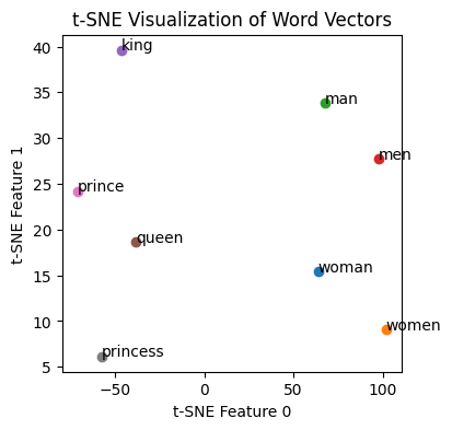
単語分散表現の可視化#

import matplotlib.pyplot as plt
from sklearn.manifold import TSNE
import numpy as np
import scienceplots
plt.style.use('science')

# List of words to visualize
words = ['woman', 'women', 'man', 'men', 'king', 'queen', 'prince', 'princess']

# Check if the words are in the model to avoid KeyError
vectors = [model[word] for word in words if word in model]

# Converting list of vectors to a numpy array
vectors_array = np.array(vectors)

# Applying t-SNE for dimensionality reduction
tsne = TSNE(n_components=2, random_state=0, perplexity=3)
vectors_tsne = tsne.fit_transform(vectors_array)

# Visualization
plt.figure(figsize=(4, 4))
for i, word in enumerate(words):
    if word in model:
        plt.scatter(vectors_tsne[i, 0], vectors_tsne[i, 1])
        plt.annotate(word, (vectors_tsne[i, 0], vectors_tsne[i, 1]))

plt.xlabel('t-SNE Feature 0')
plt.ylabel('t-SNE Feature 1')
plt.title('t-SNE Visualization of Word Vectors')
plt.show()

tensorboardで単語分散表現の可視化#

可視化の際に用いられるツールとしては、TensorFlowのツールの一つであるTensorBoardが、豊富な機能とインタラクティブな操作性を備えています。

from tensorboardX import SummaryWriter
import torch

# 分散表現・単語のリストを取得
weights = model.vectors
labels = model.index_to_key

weights = weights[:1000]
labels = labels[:1000]

writer = SummaryWriter('runs/google_embeddings')
writer.add_embedding(torch.FloatTensor(weights), metadata=labels)

上記スクリプトを実行すると、実行されたディレクトリにデータが作成されます。TensorBoardの起動時にrunsディレクトリを指定することで、変換した単語の分散表現が可視化できます。

tensorboard --logdir=runs

上記コマンドを実行した状態で http://localhost:6006/ にアクセスすると、PROJECTORのページにてグラフが確認できます。

計算社会科学のための自然言語処理

GensimによるWord2Vecの学習と使用

Contents